Rank Biserial Correlation \(r_{rb}\)#
The rank biserial correlation is a nonparametric correlation that describes the relationship between a dichotomous variable and an ordinal variable. If you have some passing familiarity with non-parametric statistical tests, then you may recognize it as being used in the Mann Whitney U test. The point of the rank biserial correlation is to indicate the proportion of favorable vs. unfavorable rank comparisons between the groups of the dichotomous variable.
An example of a use case scenario is if you wanted to compare the frustration ratings for opening a new packaging design between right-hand dominant people with left-hand dominant people.
dichotomous variable: Dominant hand
ordinal variable: Frustration
The general form of this correlation is:
\(r_{rb} = 2*\frac{(Y_{1} - Y_{0})}{n}\)
\(Y_{1}, Y_{0}\) are means of the ranks computed for data pairs.
n is the number of observations
Interpreting \(r_{rb}\)
As with many other correlation values, \(r_{rb}\) is within the range of [-1, 1], where 0 indicates no correlation.
Correlation Coefficient |
Interpretation |
|---|---|
0.00 – 0.10 |
Negligible or trivial |
0.10 – 0.30 |
Weak |
0.30 – 0.50 |
Moderate |
0.50 – 1.00 |
Strong |
Assumptions
One variable is dichotomous, and the other is ordinal.
Python Example#
To illustrate the use of the rank biserial correlation, I will generate 100 observations randomly.
# Import
import numpy as np
import pandas as pd

# Correlation coefficient
import scipy.stats as stats

# Visualizations
import matplotlib.pyplot as plt
import seaborn as sns
# Seed
np.random.seed(10)

# Create the dataframe
df = pd.DataFrame(data={'handedness': list(np.random.randint(0, 2, 100)),
                        'frustration': list(np.random.randint(1, 6, 100))})
In the above dataset assume the following:
Handedness: 0 is left hand dominant, 1 is right hand dominant.
Frustration: 1 is not at all frustrated, 5 is very frustrated.
# Turn handedness into a categorical variable
df['handedness'] = df['handedness'].astype('category')

# Look at the info
df.info()
<class 'pandas.core.frame.DataFrame'>
RangeIndex: 100 entries, 0 to 99
Data columns (total 2 columns):
 #   Column       Non-Null Count  Dtype
---  ------       --------------  -----
 0   handedness   100 non-null    category
 1   frustration  100 non-null    int64
dtypes: category(1), int64(1)
memory usage: 1.1 KB
# Describe via crosstabs
pd.crosstab(df['handedness'], df['frustration'], margins=True)
| frustration | 1 | 2 | 3 | 4 | 5 | All |
|---|---|---|---|---|---|---|
| handedness | ||||||
| 0 | 12 | 16 | 8 | 10 | 9 | 55 |
| 1 | 10 | 12 | 8 | 9 | 6 | 45 |
| All | 22 | 28 | 16 | 19 | 15 | 100 |
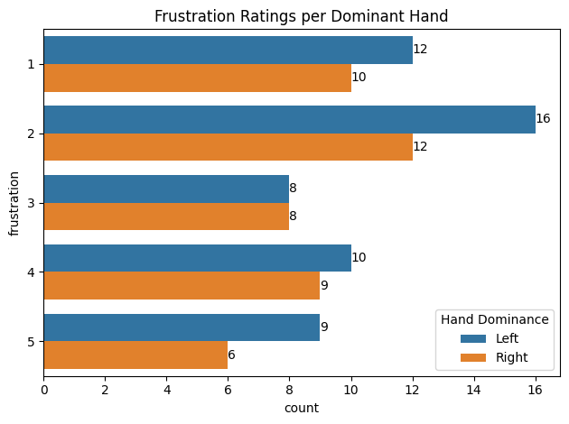
# Visualize
sns.countplot(y='frustration', hue='handedness', data=df)
# Bar annotations
plt.bar_label(plt.gca().containers[0])
plt.bar_label(plt.gca().containers[1])

# Title
plt.title('Frustration Ratings per Dominant Hand')

# Legend
plt.legend(loc='lower right', labels=['Left', 'Right'], title='Hand Dominance')

# Display
plt.tight_layout()
plt.show()
In python, the easiest way to get the rank biserial correlation is to run a Mann-Whitney U test and calculate the correlation manually.
# subset left and right
left_hand = df[df['handedness'] == 0]['frustration']
right_hand = df[df['handedness'] == 1]['frustration']

# Set up the test
u, p = stats.mannwhitneyu(left_hand, right_hand, alternative='two-sided')
# Get sizes of each group
n_left = len(left_hand)
n_right = len(right_hand)

# Calculate the r_rb
r_rb = 2 * u / (n_left * n_right) - 1

# Show
print(f'Rank biserial correlation = {r_rb} | p-value: {p}')
Rank biserial correlation = 0.007676767676767726 | p-value: 0.9490732935909326
As can be seen above, the correlation is practically non-existent. To see if it is significant, you can use p value generated from the Mann Whitney test. Unsurprisingly, it is not significant for this weak correlation.